Spectral–Spatial
Interpretation.

Which spectral channels matter, and where?

01 / THE QUESTION

A model sees six bands.
What produced its burn-scar score?
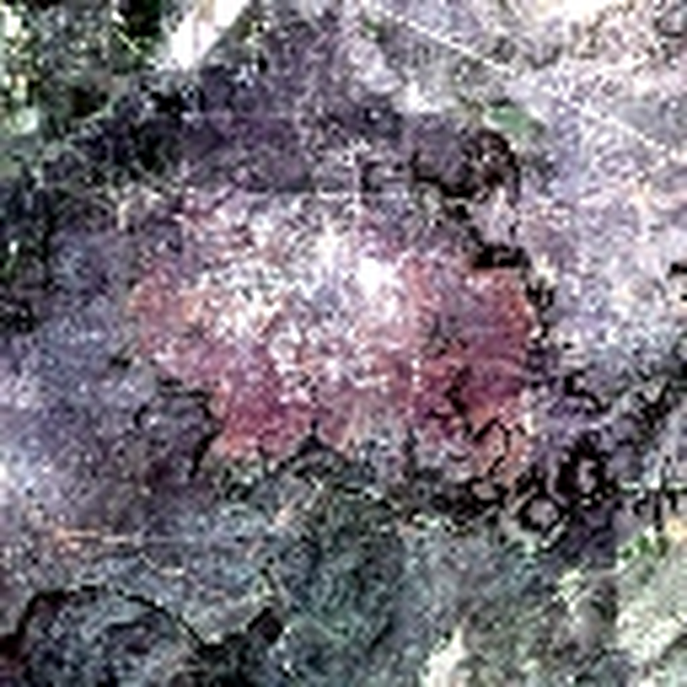
Real HLS sample 0163 satellite imageHLS BURN SCARS
Fixed target burn regionFIXED TARGET REGION
HLS image6 spectral bands
→
U-Netsegmentation
→
Burn-class logitfixed region mean
Spatial alone tells us where.
Spectral alone tells us which.
Neither tells us which band matters where.
BlueGreenRedNIRSWIR1SWIR2

The score being explained

This is an HLS Burn Scars segmentation image with six bands, Blue, Green, Red, NIR, SWIR1 and SWIR2. The trained U-Net produces burn-class logits. The explanation target is the mean logit over 2,734 pixels in the fixed ground-truth burn region.

The ground-truth mask is used to define the scalar score; it is not an input channel to the U-Net. This is a single illustrative example, not an independent localization evaluation.

Keep the surrounding image.
Change only one location.

OBSERVED IMAGEg · row 10, col 12
Original HLS satellite image
Click to move location
Only the six channels inside g change.
MEAN BASELINE
Cell masked
1.1549
OBSERVED BANDS
Cell restored
1.2065
LOCAL SCORE CHANGE+0.0516

Observed context

Choose a location in the satellite image. The score of the unmasked image stays fixed. The masked-cell score and local contrast are calculated from the saved SSI attribution for that cell; this tutorial does not run another model forward pass.

Select one order.
Play its contribution.

SELECT AN ORDER · THEN PRESS PLAY— / 05
BASELINE—
→
RESTORED—
ORDER CONTRIBUTION—
RUNNING SHAPLEY SUM

Only what you add.

Each order contributes one fifth of its effect.
CHANNELORDER CONTRIBUTIONSSUM

Shapley accumulation

Choose one order, then press Play to restore its six local channels in sequence. Each marginal score change contributes one fifth to that channel's running total. Other orders remain unchanged. Selecting an included order again removes it, and replaying an order replaces rather than duplicates its contribution.

04 / THE JOINT OBJECT

One position gives six numbers.
Repeat across the image.

Φ(g,c)256 LOCATIONS × 6 SPECTRAL BANDS
CHOOSE A BAND TO INSPECTSWIR2 · +0.7510
NEGATIVEPOSITIVE

One matrix, not two explainers

The joint attribution Phi(g,c) is a 16×16×6 tensor for this run: 256 locations and six channels. A row gives the six within-cell Shapley contributions. Fixing a channel shows how its contribution varies across locations.

Every small map here comes directly from the real 1,536-element attribution tensor, with one common diverging signed color scale. The thin colored band markers encode channel identity; red and teal within each map encode positive and negative attribution, separately from band identity.

05 / TWO VIEWS, ONE COMPUTATION

One joint matrix.
Two consistent views.
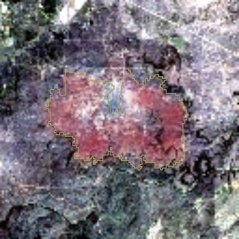
Σ CHANNELS AT EACH LOCATIONWHERE
Authentic spatial SSI map of burn-scar sample 0163
Spatial contribution
ONE COMPUTATIONΦ(g,c)
256 locations × 6 bands
Σ LOCATIONS FOR EACH BANDWHICH
Global spectral contribution

Exact aggregation of the same tensor

Spatial: S(g) = sum over c of Phi(g,c). Spectral: T(c) = sum over g of Phi(g,c). The six per-channel spatial maps are the fixed-channel slices of the same tensor.

Local efficiency is exact within each spatial cell: S(g) = f(x) - f(x with all channels of g masked). However, summing S(g) over cells need not recover the global score f(x) or a whole-image baseline contrast. For this run the sum across cells/channels is 0.874582, while the full target logit is 1.206524.

TAKEAWAYS
06 / THE EVIDENCE

Channel contributions can be spatially different.
The paper tests whether joint rankings help.

−0.532
SWIR1 VS SWIR2 SPATIAL CORRELATION

Both positive in the global total.
Different patterns across this image.

SWIR1 +0.5668SWIR2 +0.7510
PAPER RESULTS · MEAN-BASELINE JOINT DELETION ↓
CUB-2000.0088SSIbest non-SSI  0.0112
EuroSAT0.1397SSIbest non-SSI  0.2078
HLS Burn Scars0.1545SSIbest non-SSI  0.2096

SSI has the best reported mean across all three paper metrics on these datasets.

What the evidence supports

For the single HLS sample, the SWIR1 and SWIR2 signed spatial maps have Pearson correlation −0.5318 even though each band has a positive global total. At cell A, SWIR2 is +0.0730 while SWIR1 is −0.0313. These are observations for a fixed score target, not a general theorem about burn spectroscopy.

Separately, the paper reports the best mean among compared methods on joint deletion, rank-1 deletion and insertion for CUB-200, EuroSAT and HLS Burn Scars with mean and zero baselines. The displayed joint-deletion values are from the mean-baseline Table 1, not the training-split sample shown earlier.

1 / 7